- Published on
The Rules That Win on Confidence Are All About Milk
16 min read
- Authors
- Name
- Kiarash Soleimanzadeh
- https://go.kiarashs.ir/twitter



Table of Contents
- The rules that win on confidence are all about milk
- The receipts
- The one knob everybody turns
- Where Apriori spends the time
- What the FP-tree buys
- Confidence is a popularity ranking in disguise
- Five measures, five blind spots
- Lift breaks in the other direction
- Closed itemsets do nothing here
- What I would run instead
- How this was computed
- Data
- Papers referred to
The rules that win on confidence are all about milk
Two ranking metrics, one basket dataset, and a top ten that they share no entries in. Everything below was computed rather than remembered.
| Ranked first by confidence | Ranked first by lift | |
|---|---|---|
| Rule | {root vegetables, tropical fruit, yogurt} → {whole milk} | {root vegetables, tropical fruit} → {whole milk, yogurt} |
| Confidence | 0.700 | 0.271 |
| Lift | 2.74 | 4.83 |
| Baskets | 56 | 56 |
The two winners describe the same four items and rest on the same 56 receipts. Only the cut between antecedent and consequent moves.
Every tutorial on market basket analysis runs the same three steps. Pick a minimum support, run Apriori, sort the rules by confidence. I ran that pipeline on a real dataset and then took apart every step, counting what each one costs and what it throws away. The numbers in this piece all come from code executed against the data, and where a result contradicts what the textbooks promise, I have said so.
The receipts
The Groceries dataset ships with the R package arules. Its documentation describes it as 30 days of point-of-sale data from one local grocery outlet, with products rolled up to 169 categories. I parsed the CSV mirror in Python and checked my totals against the published ones: 9,835 baskets, 169 items, 43,367 item instances, density 0.02609146. All matched, including the top five item counts.
Median basket: 3 items. And 2,159 baskets hold exactly one item, so 22% of the data can never support any rule.
The shape of the data decides almost everything downstream. Whole milk appears in 2,513 baskets, better than one in four. Below that the counts fall away quickly: the fifth-ranked item, yogurt, is in 1,372 baskets, and most of the 169 categories appear in fewer than 200. A matrix that is 97.4% empty behaves very differently from the dense categorical tables that most algorithm papers benchmark on, and section 07 is where that difference stops being academic.
Table 1. Profile of the Groceries transaction database, computed from the raw CSV.
| Property | Value | Notes |
|---|---|---|
| Transactions | 9,835 | 30 days, one outlet |
| Distinct items | 169 | product categories, not SKUs |
| Item instances | 43,367 | sum of all basket sizes |
| Matrix density | 2.609% | 43,367 / (9,835 × 169) |
| Mean basket size | 4.41 | median 3, max 32 |
| Single-item baskets | 2,159 | 22.0% of all transactions |
| P(whole milk) | 0.2555 | most frequent item, 2,513 baskets |
| P(other vegetables) | 0.1935 | second, 1,903 baskets |
| P(liquor) | 0.0111 | 109 baskets, and it matters later |
The one knob everybody turns
Minimum support is usually the only parameter a tutorial touches, and every value in the plausible range looks equally defensible written down. They are not equally defensible. Moving from 5% to 0.1% support multiplies the frequent itemsets by 435 and the rules by nearly five thousand.
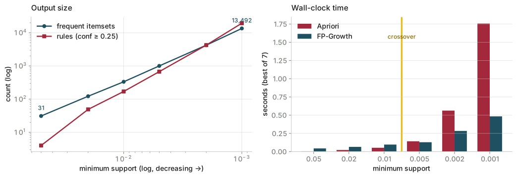
At 5% support the search returns 31 itemsets: 28 single items and three pairs. That is not a data mining result, it is a shopping list. At 0.1% the search returns 13,492 itemsets running up to size six, and a confidence filter of 0.25 turns them into 19,390 rules. No analyst reads 19,390 rules.
0.1% support means 10 baskets. Every pattern at that threshold rests on ten receipts out of 9,835.
The threshold also controls how deep the patterns go, and the depth arrives suddenly. At 1% support nothing larger than a triple survives. Drop to 0.2% and quadruples appear; drop to 0.1% and you get 3,137 quadruples, 376 quintuples and ten six-item sets. Those long itemsets are where the combinatorics live, and they are what makes the choice of algorithm start to matter.
Table 2. Frequent itemsets by size, with the rule count each threshold produces at confidence ≥ 0.25. Times are the best of seven runs of the mlxtend implementations, single-threaded.
| Min support | k=1 | k=2 | k=3 | k=4 | k=5 | k=6 | Total | Rules | Apriori | FP-Growth |
|---|---|---|---|---|---|---|---|---|---|---|
| 0.05 | 28 | 3 | 0 | 0 | 0 | 0 | 31 | 4 | 0.005 s | 0.044 s |
| 0.02 | 59 | 61 | 2 | 0 | 0 | 0 | 122 | 49 | 0.022 s | 0.065 s |
| 0.01 | 88 | 213 | 32 | 0 | 0 | 0 | 333 | 170 | 0.053 s | 0.097 s |
| 0.005 | 120 | 605 | 264 | 12 | 0 | 0 | 1,001 | 673 | 0.142 s | 0.129 s |
| 0.002 | 147 | 1,674 | 1,991 | 395 | 16 | 0 | 4,223 | 4,238 | 0.563 s | 0.284 s |
| 0.001 | 157 | 2,981 | 6,831 | 3,137 | 376 | 10 | 13,492 | 19,390 | 1.758 s | 0.484 s |
Both implementations returned identical itemset counts at every threshold, which is the check that the comparison is measuring speed and not correctness.
Where Apriori spends the time
Apriori generates candidates of size k by joining pairs of frequent (k−1)-itemsets that share their first k−2 items, discards any candidate with an infrequent subset, then makes a pass over the database to count what remains. To see the cost directly I wrote the textbook version and instrumented it, rather than trusting a library that vectorises the counting away. It reproduces the library's frequent itemset counts exactly, so the accounting below describes the same search.
90.8% counted for nothing. Of the 10,919 candidates Apriori counts at 0.5% support, that share turn out to be infrequent.
At 0.5% support the algorithm counts 10,919 candidates against the database and keeps 1,001. The waste is concentrated at level two, where there is nothing to prune: 120 frequent single items generate all 7,140 pairs, and 605 survive. Downward closure cannot help at k=2 because every subset of a pair is a frequent single item by construction. It starts earning its keep at k=3, where it discards 555 of 4,013 joined triples before any counting happens.
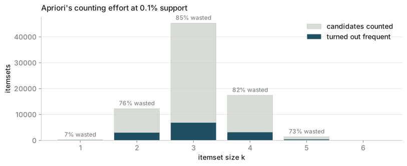
Drop to 0.1% and the picture stretches without changing shape. The join at level three produces 62,217 triples; subset pruning throws out 16,913 of them, or 27%, and the remaining 45,304 all get counted. Across the whole run, 76,595 candidates are counted to find 13,492 itemsets. The pruning rule that Apriori is named for is doing real work and is still not the dominant term.
Table 3. Level-by-level accounting for textbook Apriori at 0.1% minimum support (10 baskets). "Joined" is what the candidate join produces, "pruned" is what downward closure removes before counting.
| k | Joined | Pruned | Counted | Frequent | Hit rate |
|---|---|---|---|---|---|
| 1 | — | — | 169 | 157 | 92.9% |
| 2 | 12,246 | 0 | 12,246 | 2,981 | 24.3% |
| 3 | 62,217 | 16,913 | 45,304 | 6,831 | 15.1% |
| 4 | 24,409 | 6,970 | 17,439 | 3,137 | 18.0% |
| 5 | 2,430 | 1,023 | 1,407 | 376 | 26.7% |
| 6 | 47 | 17 | 30 | 10 | 33.3% |
| Total | 101,349 | 24,923 | 76,595 | 13,492 | 17.6% |
What the FP-tree buys
FP-Growth replaces candidate generation with a data structure. It reads the database twice: once to count single items, once to insert each basket, with its items sorted by descending global frequency, into a prefix tree. Baskets sharing a prefix share nodes. After that the database is never touched again, and the mining runs recursively over conditional trees built from the node links.
Restricted to the three most frequent items, the whole database collapses to seven nodes. Of the 9,835 baskets, 4,689 contain at least one of whole milk, other vegetables and rolls/buns, and between them they carry 6,225 item instances. All of it fits below.
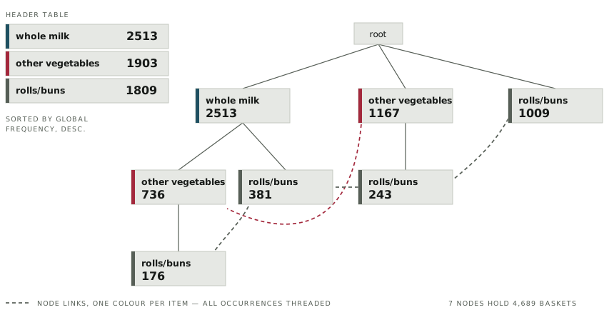
Building that tree is not free, and the benchmark in table 2 shows where the bill comes due. At 5% support FP-Growth spends 44 milliseconds constructing a tree for a search that mlxtend's Apriori finishes in 5, because that Apriori is not the textbook loop: it counts candidates with vectorised operations over a boolean matrix, which is very fast while the candidate sets stay small. The tree pays for itself at 0.5% support and wins by 3.6× at 0.1%.
Crossover: 0.5% support. Above it the tree is overhead; below it, it is the reason the search finishes.
Two caveats on that number. It compares two implementations in one library on a single vCPU, not the algorithms in the abstract, and a C implementation of either would move the crossover. And 9,835 baskets is small; the gap widens with the database because Apriori's cost scales with passes over the data while FP-Growth's tree, once built, does not.
Confidence is a popularity ranking in disguise
Set minimum support to 0.5% and minimum confidence to 0.25, and the search returns 673 rules. Of those, 221 have {whole milk} as their consequent and 178 have {other vegetables}. Two items out of 169 account for 59% of the output.
The reason is arithmetic, not merchandising. Confidence is P(B|A), and its ceiling is set by how common B is. Lift divides that same quantity by P(B), so for a fixed consequent the two metrics are the same number on different scales. Sorting a mixed pile of rules by confidence therefore sorts them mostly by the base rate of whatever sits on the right-hand side, and whole milk has the highest base rate in the dataset.
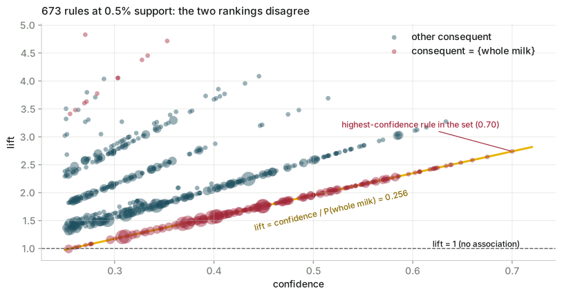
Fig 4 makes the structure literal. The red points are one ray, the flattest one in the plot, and the confidence ranking simply walks it from the right. Nine of the top ten rules by confidence end in whole milk; the tenth ends in other vegetables. The top ten by lift contains none of them. Not one rule appears in both lists.
Shared entries: 0. Between the top ten by confidence and the top ten by lift, from the same 673 rules.
Table 4. The two rankings side by side, 673 rules at 0.5% support and confidence ≥ 0.25. Rules are listed in each metric's own order.
| Rank | Ranked by confidence | Conf | Lift | Ranked by lift | Conf | Lift |
|---|---|---|---|---|---|---|
| 1 | root veg, tropical fruit, yogurt → whole milk | 0.700 | 2.74 | root veg, tropical fruit → whole milk, yogurt | 0.271 | 4.83 |
| 2 | other veg, pip fruit, root veg → whole milk | 0.675 | 2.64 | pip fruit, root veg → other veg, whole milk | 0.353 | 4.72 |
| 3 | butter, whipped/sour cream → whole milk | 0.660 | 2.58 | root veg, tropical fruit → other veg, whole milk | 0.333 | 4.45 |
| 4 | pip fruit, whipped/sour cream → whole milk | 0.648 | 2.54 | citrus fruit, root veg → other veg, whole milk | 0.328 | 4.38 |
| 5 | butter, yogurt → whole milk | 0.639 | 2.50 | citrus fruit, other veg, whole milk → root veg | 0.445 | 4.09 |
| 6 | butter, root veg → whole milk | 0.638 | 2.50 | root veg, whipped/sour cream → other veg, whole milk | 0.304 | 4.06 |
| 7 | curd, tropical fruit → whole milk | 0.634 | 2.48 | butter, other veg → whipped/sour cream | 0.289 | 4.04 |
| 8 | citrus fruit, root veg, whole milk → other veg | 0.633 | 3.27 | herbs → root vegetables | 0.431 | 3.96 |
Seven of the eight highest-confidence rules end in whole milk. The lift ranking finds {herbs} → {root vegetables}, a rule that covers 69 baskets and never comes close to the confidence top hundred.
Five measures, five blind spots
Take one rule and read it through every standard measure. {butter, yogurt} → {whole milk} holds in 92 baskets; butter and yogurt appear together in 144; whole milk appears in 2,513. Each measure below is computed from those three counts and the database size.
Table 5. Interest measures for {butter, yogurt} → {whole milk}, N = 9,835, n(A) = 144, n(B) = 2,513, n(A∩B) = 92.
| Measure | Definition | Value | What it cannot see |
|---|---|---|---|
| Support | P(A∩B) | 0.0094 | Whether the co-occurrence beats chance at all |
| Confidence | P(B|A) | 0.639 | P(B). A common consequent inflates every rule that points at it |
| Lift | P(B|A) / P(B) | 2.500 | How many baskets the rule covers, and how unstable the estimate is when it covers few |
| Leverage | P(A∩B) − P(A)P(B) | 0.0056 | Rare-item structure: it is bounded by 0.25 and squeezes small items together near zero |
| Conviction | (1 − P(B)) / (1 − P(B|A)) | 2.062 | Nothing at confidence 1, where it is undefined |
| Fisher p | one-sided, 2×2 table | 2.0×10⁻²² | Effect size, and the fact that 100,000 other rules were tested |
Leverage is the one that gets least attention and behaves best across a mixed set of rules. It is an absolute deviation from independence rather than a ratio, so a rule cannot score highly on a handful of baskets. Its top of the list on this data is {root vegetables} → {other vegetables} at 0.0263, covering 466 baskets, followed by the whole milk and other vegetables pair at 0.0254 across 736. Those are the two pairs that actually move volume in this shop.
Lift breaks in the other direction
Push support down to 0.1% and lift finds the patterns confidence never will. The strongest is {bottled beer, red/blush wine} → {liquor} at lift 35.7. Liquor is in 109 baskets, beer and wine appear together in 48, and 19 of those 48 also contain liquor. As a piece of retail intelligence this is worth more than every milk rule in table 4 combined.
It also rests on 19 receipts. The Wilson 95% interval on that confidence of 0.396 runs from 0.270 to 0.537, which puts the lift somewhere between 24 and 48. The next nine rules by lift each rest on exactly ten baskets, and one of them, {oil, tropical fruit, whole milk} → {other vegetables, root vegetables, yogurt}, has a lift interval from 18 to 46. You cannot plan a planogram around a number with that much room in it.
90.6% survive BH at q = 0.05, out of the 101,430 rules with lift above 1. Significance testing is not the filter people hope it is.
The obvious response is a significance test, so I ran one: a one-sided Fisher exact test on every rule's 2×2 table, with Benjamini-Hochberg correction across the whole family. At 0.1% support, 101,430 rules have lift above 1 and 91,886 of them survive at q = 0.05. At 0.5% support, 2,662 of 2,868 survive. The test is doing almost nothing, because with 9,835 baskets and items appearing 50 to 2,500 times, even weak dependencies clear the bar easily. What survives correction is not what is worth acting on.
The rule that runs the opposite way is {sausage} → {whole milk}: 294 baskets, confidence 0.318, Fisher p of 4×10⁻⁶, and a lift of 1.25. Statistically real, commercially empty. Sausage buyers buy milk at almost exactly the rate everyone else does.
Closed itemsets do nothing here
The standard cure for output volume is to mine closed itemsets instead of all frequent ones. An itemset is closed when no superset has the same support, so the closed sets carry all the support information with none of the duplication. Textbooks introduce this as a general reduction. On Groceries it is not a reduction at all.
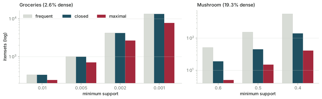
At 1%, 0.5% and 0.2% support, every single frequent itemset on Groceries is closed. At 0.1% support, 13,464 of 13,492 are. Closure only collapses an itemset when some superset occurs in exactly the same baskets, and in a matrix that is 97.4% empty, exact co-occurrence of that kind is close to impossible.
Run the same computation on Mushroom, 8,124 records with 23 attribute-value pairs each and a density of 19.3%, and closure does what the textbooks describe: 51 frequent itemsets at 60% support reduce to 19 closed ones, and 565 at 40% support reduce to 140. Closed itemset mining is a dense-data optimisation that got written up as a general one.
Table 6. Itemset compression against database density. Closed and maximal counts were computed directly; the closure test checks each itemset against its immediate supersets.
| Database | Density | Min support | Frequent | Closed | Maximal |
|---|---|---|---|---|---|
| Groceries | 2.6% | 0.01 | 333 | 333 (100%) | 243 (73%) |
| 0.005 | 1,001 | 1,001 (100%) | 708 (71%) | ||
| 0.002 | 4,223 | 4,223 (100%) | 2,675 (63%) | ||
| 0.001 | 13,492 | 13,464 (99.8%) | 7,794 (58%) | ||
| Mushroom | 19.3% | 0.6 | 51 | 19 (37%) | 5 (10%) |
| 0.5 | 153 | 45 (29%) | 15 (10%) | ||
| 0.4 | 565 | 140 (25%) | 41 (7%) |
Maximal itemsets do compress Groceries, down to 58% of the frequent sets at 0.1% support, but they are the wrong tool for rule mining: a maximal set keeps no support counts for its subsets, so you cannot compute confidence or lift from it without going back to the data.
Pruning redundant rules helps about as little. Dropping every rule whose antecedent has a strict subset achieving equal or higher confidence for the same consequent removed 27 of the 673 rules at 0.5% support. Four percent. The 673 rules are not mostly duplicates of each other; they are mostly small variations that each cover a slightly different set of baskets, and no syntactic rule collapses them.
What I would run instead
None of the above says the technique is broken. It says the default pipeline hides its own failure modes, and four changes fix most of it.
- Fix the consequent before you rank. Decide what you are trying to predict, filter to rules with that item on the right, then sort by confidence. Within one consequent, confidence and lift give identical orderings and both are meaningful. The disagreement in table 4 exists only because the pile was mixed.
- If the pile must stay mixed, rank by leverage. It is an absolute deviation rather than a ratio, so a ten-basket coincidence cannot reach the top. Report lift alongside it, never on its own.
- Set an absolute minimum count, not a percentage. A fraction that sounds conservative at 0.1% means ten receipts. Pick a count that the business would act on, 50 or 100, and derive the support threshold from it. The percentage will look absurdly high, and that is the point.
- Choose the algorithm from the threshold, not from the literature. Above roughly 0.5% support on data this size, level-wise counting wins and the FP-tree is pure overhead. Below it, build the tree. And skip closed itemset mining on sparse baskets entirely; measure the closure ratio once before you commit to it.
The version of this analysis worth trusting also has an ingredient I do not have: a second month of receipts. Every number here is a point estimate from a single 30-day window, and the honest test of {bottled beer, red/blush wine} → {liquor} is whether those 19 baskets are still there in November.
How this was computed
Python 3.12 with pandas 3.0.2, numpy 2.4.4, scipy 1.17.1 and mlxtend 0.25.0, on a single Intel Xeon vCPU at 2.10 GHz. Timings are the fastest of seven runs. The instrumented Apriori is my own implementation of the F_{k−1} × F_{k−1} join with downward-closure pruning; it reproduces mlxtend's frequent itemset counts exactly at every threshold tested. Closure was tested against immediate supersets only, which is sufficient by monotonicity. Confidence intervals are Wilson score intervals at 95%.
Data
Groceries, distributed with the R package arules and provided by Michael Hahsler, Kurt Hornik and Thomas Reutterer (2006). Read from the CSV mirror at https://github.com/stedy/Machine-Learning-with-R-datasets. Mushroom, originally from the UCI Machine Learning Repository, read from the same mirror and encoded as attribute=value items.
Papers referred to
- Agrawal, Imieliński and Swami, "Mining association rules between sets of items in large databases", SIGMOD 1993.
- Agrawal and Srikant, "Fast algorithms for mining association rules", VLDB 1994.
- Han, Pei and Yin, "Mining frequent patterns without candidate generation", SIGMOD 2000.
- Brin, Motwani, Ullman and Tsur, "Dynamic itemset counting and implication rules for market basket data", SIGMOD 1997.
- Pasquier, Bastide, Taouil and Lakhal, "Discovering frequent closed itemsets for association rules", ICDT 1999.
- Benjamini and Hochberg, "Controlling the false discovery rate", JRSS-B 1995.
- Webb, "Discovering significant patterns", Machine Learning 2007.