Probability and Statistics for AI

A training run is a chain of expectations that nobody can compute. The loss is an expectation over a data distribution you have only samples from. The gradient is an expectation over a minibatch, and in a latent-variable model over the latent as well. The benchmark number at the end is an expectation over a finite evaluation set and over a random seed. Each link is estimated, and each estimate has a variance that somebody picked by accident.

This is a reference for all of it. The organizing claim, which the rest of the piece argues for, is that four questions carry most of the weight: which distribution is this expectation taken over, what is the variance of the estimator I replaced it with, which way does my divergence point, and how many samples stand behind the number I am about to publish. Everything else is machinery in service of those four.

Twenty-three figures follow, and every one is a computation rather than a drawing. Where a number appears in the text it came out of the code that produced the adjacent plot. Sections are self-contained enough to be read out of order; the parts are ordered so that later ones can use earlier notation.

Part I. Foundations

Where measure theory actually bites

The formal object is a triple $(\Omega, \mathcal{F}, P)$: a set of outcomes, a $\sigma$-algebra of events closed under complement and countable union, and a countably additive measure with $P(\Omega)=1$. A random variable is a measurable map $X : \Omega \to \mathbb{R}^d$, and its distribution is the pushforward $P \circ X^{-1}$.

You can do a great deal of machine learning without writing that down. It earns its keep in four places.

Change of variables is the first. If $f$ is a diffeomorphism and $y = f(x)$,

Normalizing flows are that identity turned into an architecture. It is also why a density can exceed one, and why a number a continuous model calls a probability is not one.

The Radon-Nikodym derivative is the second. Importance weights, likelihood ratios in off-policy learning, and KL divergence are all $dP/dQ$, and each is undefined when $P$ is not absolutely continuous with respect to $Q$. A training example your proposal assigns zero mass to does not produce a large weight, it produces an object that does not exist.

Conditional expectation is the third. $E[Y \mid X]$ is the projection of $Y$ onto the closed subspace of square-integrable $X$-measurable functions, which is why the conditional mean minimizes squared error, and why a network trained with MSE converges to it rather than to any individual target. Train the same architecture with cross entropy and you get the conditional distribution instead.

Infinite-dimensional objects are the fourth: Gaussian processes, Dirichlet processes, diffusion limits, anything where "the density" does not exist and the Kolmogorov extension theorem is doing real work.

Outside those, the scaffolding can stay in the background.

Conditioning, Bayes, and exchangeability

Three rules do nearly all the manipulation. The chain rule factors any joint distribution in any order, $p(x_1,\dots,x_n) = \prod_i p(x_i \mid x_{\lt i})$, and autoregressive models are this and nothing more. The law of total probability marginalizes, $p(x) = \sum_z p(x \mid z) p(z)$, and every latent-variable model is an instance. Bayes' rule inverts a conditional:

The denominator is the reason inference is hard. Everything in the approximate-inference section exists because that integral is intractable.

Independence, $p(x,y) = p(x)p(y)$, is strictly stronger than zero correlation: $Y = X^2$ with $X$ symmetric has correlation zero and complete dependence. Conditional independence, $X \perp Y \mid Z$, is the weaker and far more useful notion, because it is what graphical models encode and what lets a joint distribution over a thousand variables be written down at all.

Exchangeability deserves more attention than it gets in machine learning. A sequence is exchangeable if its joint distribution is invariant under permutation, which is weaker than i.i.d. De Finetti's theorem says an infinite exchangeable binary sequence is a mixture of i.i.d. sequences, $p(x_{1:n}) = \int \prod_i \theta^{x_i}(1-\theta)^{1-x_i} \,\pi(\theta)\,d\theta$, which is the cleanest argument for why a Bayesian prior is not optional but implied. Exchangeability is also the exact assumption conformal prediction needs, and the exact assumption that fails when your test set was scraped after your training set.

Random variables, transformations, and sampling anything

A distribution is specified by its CDF $F(x) = P(X \le x)$, and by a PMF or density where one exists. Three transformation facts cover most practical needs.

Inverse CDF sampling: if $U \sim \mathrm{Uniform}(0,1)$ then $F^{-1}(U) \sim F$. This is how exponential and Cauchy samplers are written, and why quantile functions matter.

Rejection sampling: to sample $p$ given a proposal $q$ with $p(x) \le M q(x)$, draw $x \sim q$ and accept with probability $p(x)/(M q(x))$. The acceptance rate is $1/M$, which degrades exponentially in dimension and is why nobody uses it above a handful of dimensions.

The Gumbel-max trick: if $g_i$ are i.i.d. standard Gumbel then $\arg\max_i (\log \alpha_i + g_i)$ is a draw from the categorical distribution with probabilities proportional to $\alpha_i$. Softmax sampling is usually implemented this way, and relaxing the argmax to a softmax gives the Gumbel-softmax gradient estimator.

Two moment identities that get used constantly. The law of total expectation, $E[Y] = E[E[Y \mid X]]$, and the law of total variance,

The second is the formal statement that conditioning on something can only reduce expected variance, which is the whole content of Rao-Blackwellization and most variance-reduction schemes.

The distributions worth knowing cold

Not a catalogue for its own sake: each of these shows up as a modelling choice with consequences.

Bernoulli and categorical are the output distributions of classifiers, and their log likelihoods are exactly binary and multiclass cross entropy. Binomial and multinomial are their counts. Poisson, $p(k) = \lambda^k e^{-\lambda}/k!$, models counts with mean equal to variance, and real count data is usually overdispersed, which is what negative binomial fixes. Geometric and exponential are the memoryless waiting times.

Gaussian is the maximum-entropy distribution for fixed mean and covariance, closed under linear maps, marginalization, conditioning, and convolution, and it is the limit in the CLT. Those closure properties, not any claim about nature, are why it is everywhere.

Laplace has heavier tails and its MAP estimate is $L_1$ regularization. Student-$t$ with $\nu$ degrees of freedom interpolates between Cauchy and Gaussian and is the standard robust replacement for a Gaussian likelihood: it is a scale mixture of Gaussians, which makes it easy to fit by EM. Cauchy has no mean, which matters more than it sounds.

Beta is the conjugate prior for Bernoulli, Dirichlet for categorical, Gamma for a Poisson rate, and Normal-Inverse-Wishart for a Gaussian with unknown mean and covariance. Conjugacy means the posterior stays in the family, so updating is arithmetic on counts:

Dirichlet is also the smoothing in a smoothed n-gram model, and the topic prior in LDA. Chi-squared, $F$, and $t$ are the sampling distributions that classical tests are built on. Von Mises-Fisher is the distribution on the sphere, which is what a normalized embedding lives on, and it is the right likelihood for cosine-similarity models.

Gumbel and the generalized extreme value family govern maxima, which is what best-of-$n$ sampling produces.

Exponential families and sufficiency

A family is exponential if

with natural parameter $\eta$, sufficient statistic $T(x)$, and log-partition $A(\eta)$. Almost everything in the previous section is a member.

Two properties make this more than taxonomy. First, $A$ generates moments: $\nabla_\eta A(\eta) = E[T(X)]$ and $\nabla^2_\eta A(\eta) = \operatorname{Cov}[T(X)]$, so $A$ is convex and the map from natural to mean parameters is invertible. Second, the MLE is moment matching: setting the gradient of the log likelihood to zero gives $E_{\hat\eta}[T(X)] = \frac{1}{n}\sum_i T(x_i)$, and nothing else about the data matters. That is the Fisher-Neyman factorization: $T(x)$ is sufficient, and a fixed-dimension sufficient statistic exists only for exponential families (Pitman-Koopman-Darmois).

Softmax classification is the categorical exponential family with logits as natural parameters, which is why its loss is convex in the logits, why temperature scaling is a natural-parameter rescaling, and why the gradient of cross entropy is the elegant $\hat{p} - y$. Restricted Boltzmann machines, conditional random fields, and every energy-based model are exponential families with an intractable $A(\eta)$, and the whole difficulty of training them is that one term.

The multivariate Gaussian

Worth its own section because so much reduces to it. With $x \sim \mathcal{N}(\mu, \Sigma)$,

and the exponent is the squared Mahalanobis distance. Partition $x = (x_1, x_2)$ and both the marginal and the conditional stay Gaussian:

The conditional mean is linear in $x_2$ and the conditional covariance does not depend on $x_2$ at all. Gaussian process regression is that formula applied to a covariance built from a kernel; the Kalman filter is that formula applied twice per timestep; linear regression with Gaussian noise is the same object again.

The precision matrix $\Lambda = \Sigma^{-1}$ encodes conditional independence directly: $\Lambda_{ij} = 0$ if and only if $x_i \perp x_j$ given everything else. That is the Gaussian graphical model, and it is why sparse precision estimation (the graphical lasso) is structure learning.

Sampling uses the Cholesky factor $\Sigma = LL^{\top}$ and $x = \mu + Lz$, which is the reparameterization trick in its original form. Whitening is the inverse operation, and batch normalization is a crude diagonal version applied to activations.

Limit theorems, and where they fail

The weak law of large numbers says $\bar X_n \to \mu$ in probability; the strong law gives almost-sure convergence. Both need a finite mean and nothing else. The central limit theorem says

and the Berry-Esseen theorem bounds the error of the approximation by $C\rho/(\sigma^3\sqrt{n})$ with $\rho = E|X-\mu|^3$, so skewed summands converge more slowly. The delta method extends this to smooth functions: if $\sqrt{n}(\hat\theta - \theta) \to \mathcal{N}(0,\sigma^2)$ then $\sqrt{n}(g(\hat\theta) - g(\theta)) \to \mathcal{N}(0, g'(\theta)^2\sigma^2)$, which is how you get a standard error for a ratio, an F1 score, or a log-odds.

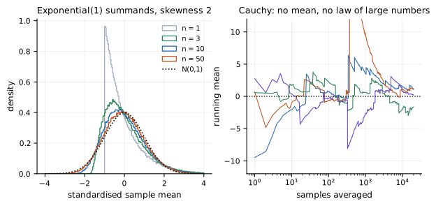
The right panel is the practical warning. Heavy tails break the law of large numbers, and machine learning is full of heavy tails: gradient norms, attention weights, token frequencies, loss on a hard subset, revenue per user. A sample mean of a quantity with infinite variance still converges, but the CLT rate does not apply and confidence intervals built from it are wrong. Check tails before averaging.

Four modes of convergence show up and are worth keeping straight: almost sure implies in probability implies in distribution, and $L^p$ convergence implies in probability. Slutsky's theorem lets you replace a consistent variance estimate inside a limiting distribution, which is what licenses plugging $\hat\sigma$ into a $z$-interval. The continuous mapping theorem says convergence survives continuous functions.

Life in high dimensions

Intuition built in two or three dimensions is not merely imprecise in a thousand, it is inverted.

Concentration of measure: for $x \sim \mathcal{N}(0, I_d)$, $\|x\|$ concentrates sharply around $\sqrt{d}$ with fluctuations of order one, independent of $d$. The mass of a high-dimensional Gaussian is not near the mode; it is on a thin shell. This is why interpolating between two latent codes along a straight line passes through a low-density region, and why spherical interpolation is the standard fix.

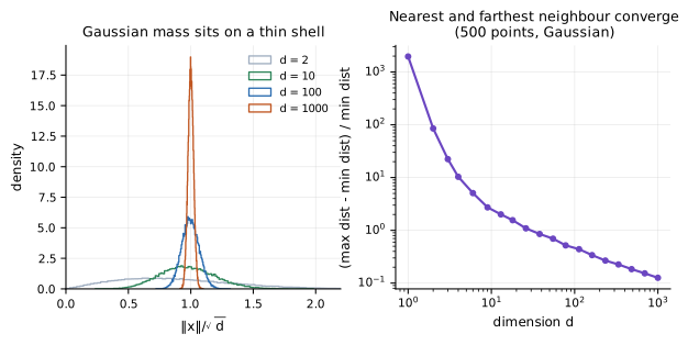
The right panel is the curse of dimensionality stated precisely. When all pairwise distances become comparable, a nearest neighbour is barely nearer than a random point, and any method whose output depends on that ranking degrades. Real data is saved by lying on a lower-dimensional manifold; the effective dimension, not the ambient one, is what matters, which is the entire premise of representation learning.

Random matrices. For an $n \times p$ matrix with i.i.d. entries of variance one, the eigenvalues of $\frac{1}{n}X^{\top}X$ follow the Marchenko-Pastur law with support $[(1-\sqrt{\lambda})^2, (1+\sqrt{\lambda})^2]$ for $\lambda = p/n$. This is why a sample covariance from $n \approx p$ samples is badly conditioned even when the truth is the identity, why shrinkage estimators help, and why the double descent peak appears exactly at $p = n$: the smallest eigenvalue touches zero there.

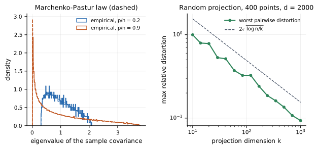
The Johnson-Lindenstrauss lemma says $k = O(\log n / \epsilon^2)$ dimensions suffice to preserve all pairwise distances among $n$ points to relative error $\epsilon$, with no dependence on the original dimension. Random projections, LSH, sketching, and the reason a 768-dimensional embedding can stand in for a much larger space all follow from it. Matrix concentration inequalities (Tropp's matrix Bernstein and friends) extend the scalar bounds of the next part to sums of random matrices, and are the tool behind spectral-norm bounds on random initializations.

Initialization scaling is the same calculation in disguise. A layer $W x$ with $W_{ij} \sim \mathcal{N}(0, \sigma^2)$ maps a unit-norm input to something of squared norm $\approx \sigma^2 d_{\text{in}}$, so keeping activations from exploding or vanishing across depth requires $\sigma^2 = 1/d_{\text{in}}$ for linear or tanh layers and $2/d_{\text{in}}$ for ReLU, which absorbs the factor of two lost by zeroing half the units. He and Glorot initialization are variance propagation, not folklore.

Part II. Estimation and computation

Expectations you cannot compute

Almost every quantity of interest is $\mu = E_p[f(X)]$ with a $p$ you can sample and an integral you cannot do. The Monte Carlo estimator

has error falling like $n^{-1/2}$ regardless of dimension, which is what makes high-dimensional integration possible at all, and it is also brutally slow: ten times the accuracy costs a hundred times the samples.

Importance sampling reweights a different proposal,

staying unbiased for any $q$ covering the support while the variance depends entirely on the choice.

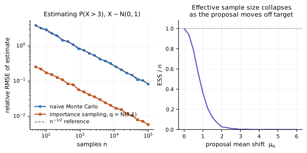
The panels disagree deliberately. Effective sample size,

diagnoses the weights alone. The proposal centred at 3 has near-zero ESS against a standard normal target and is still the better estimator here by a factor of fourteen in RMSE. ESS answers "could these weights estimate a typical expectation", not "are they good for my integrand", and reporting it as a verdict points the wrong way exactly when importance sampling is working. Self-normalized importance sampling, which divides by $\sum_i w_i$ because $p$ is known only up to a constant, is biased at finite $n$ and consistent, and it is what off-policy RL and RLHF reweighting actually use.

Control variates replace $f$ with $f - c(g - E[g])$ for a $g$ with known mean, with optimal $c$ equal to the regression coefficient of $f$ on $g$. Antithetic variates use negatively correlated pairs. Rao-Blackwellization integrates out analytically whatever has a closed form, and the law of total variance guarantees it never increases variance. Stratification and common random numbers are the other two standard tricks, and common random numbers in particular is underused in benchmarking: comparing two methods on the same seeds removes the shared variance.

Differentiating through randomness

Variational inference, policy gradients, and every latent-variable model need $\nabla_\theta E_{q_\theta}[f(X)]$ where $\theta$ sits in the distribution. Two estimators, very different behaviour.

The log-derivative identity $\nabla_\theta q_\theta = q_\theta \nabla_\theta \log q_\theta$ gives the score-function estimator,

which is REINFORCE (Williams, 1992). It requires nothing of $f$ but evaluation, so it works for discrete variables, non-differentiable rewards, and black-box simulators.

The pathwise estimator requires $X = g(\epsilon,\theta)$ with $\epsilon$ from a fixed distribution and gives

For a Gaussian, $g = \mu_\theta + \sigma_\theta \epsilon$. This is the reparameterization trick of Kingma and Welling (2013) and Rezende, Mohamed and Wierstra (2014).

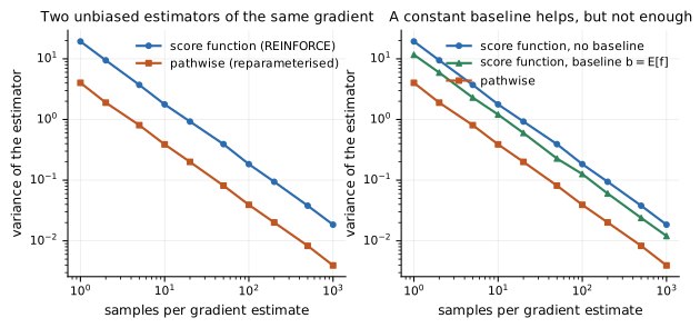
Subtracting a baseline leaves the score-function estimator unbiased because $E_{q_\theta}[\nabla_\theta \log q_\theta] = 0$. In Figure 5 a constant baseline closes less than half the gap, which is why practical systems use learned state-dependent baselines, and why actor-critic methods exist at all: the critic is a variance reduction device before it is anything else. For discrete variables the Gumbel-softmax relaxation (Jang, Gu and Poole, 2016; Maddison, Mnih and Teh, 2016) buys pathwise gradients at the cost of bias, and estimators like REBAR and RELAX buy back unbiasedness with a learned control variate.

How wrong can an average be

Every reported metric is a sample mean, and concentration inequalities bound the distance to the truth on a ladder of assumptions.

Markov needs only non-negativity, $P(X \ge a) \le E[X]/a$. Chebyshev adds a variance, $P(|X-\mu| \ge k\sigma) \le 1/k^2$. Hoeffding (1963) adds boundedness and buys an exponential rate: for independent $X_i \in [a,b]$,

Bernstein replaces the range with the variance,

which is far tighter for rare events: a task where the model is right 99% of the time has $\sigma^2 \approx 0.01$, not $0.25$. McDiarmid generalizes Hoeffding to any function of independent variables with bounded differences, and is the workhorse behind uniform convergence. The modern packaging is sub-Gaussian and sub-exponential tail conditions, which cover unbounded variables and compose cleanly; Vershynin (2018) and Boucheron, Lugosi and Massart (2013) are the references.

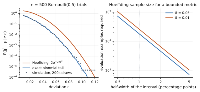
Inverting Hoeffding gives the number worth memorizing. For a metric in $[0,1]$, a two-sided interval of half-width $\epsilon$ at confidence $1-\delta$ needs

which is 18,444 examples at $\epsilon = 0.01$, $\delta = 0.05$. Most public benchmarks are one to two orders of magnitude smaller, so a one-point gap on a thousand-item test set is not distinguishable from noise by any distribution-free argument. Bernstein, the exact Clopper-Pearson interval, and Wilson intervals all do better near the boundary, and none of them rescues a 250-item evaluation.

All of this holds for a fixed hypothesis. The moment the hypothesis was chosen using the same data, it fails, which is the subject of the generalization section.

Point estimation and decision theory

An estimator is a function of the data; statistical decision theory asks which one to pick. Fix a loss $L(\theta, \hat\theta)$ and define the risk $R(\theta, \hat\theta) = E_{\theta}[L(\theta, \hat\theta(X))]$. Frequentists compare risk functions, which are curves rather than numbers, so the comparison is partial: an estimator is admissible if nothing dominates it everywhere, minimax if it minimizes worst-case risk. Bayesians integrate risk against a prior and get a single number, and the minimizer is the Bayes estimator, which for squared loss is the posterior mean, for absolute loss the posterior median, and for 0-1 loss the posterior mode.

Maximum likelihood, $\hat\theta_n = \arg\max_\theta \sum_i \log p_\theta(x_i)$, is consistent and asymptotically efficient under regularity:

The Cramér-Rao bound says no unbiased estimator beats $I(\theta)^{-1}/n$. Amari's natural gradient (1998) is descent preconditioned by $I(\theta)^{-1}$, and K-FAC and its relatives are attempts to approximate that inverse at scale.

Method of moments is the older alternative: match sample moments to population ones and solve. It is usually less efficient and often much easier, and generalized method of moments is the workhorse of econometrics.

Two results deserve to be better known in machine learning. Rao-Blackwell: conditioning any estimator on a sufficient statistic weakly reduces its risk under any convex loss, which formalizes "integrate out what you can". And Stein's paradox: for $d \ge 3$, the sample mean of a multivariate Gaussian is inadmissible under squared loss, and the James-Stein estimator that shrinks it toward an arbitrary point dominates it everywhere. Shrinkage is not a Bayesian preference, it is a theorem, and it is the cleanest argument that regularization improves estimation even when the prior is wrong.

Robustness is the other half. The mean has an influence function that is unbounded, so a single outlier moves it arbitrarily; the median does not. Huber loss interpolates, and gradient clipping is the same idea applied to the score rather than the residual.

Resampling: bootstrap, jackknife, permutation

The bootstrap (Efron, 1979) estimates the sampling distribution of any statistic by resampling the data with replacement and recomputing. It needs no formula for the standard error, which is why it is the right default for BLEU, F1, AUC, calibration error, or any metric that is not a plain average.

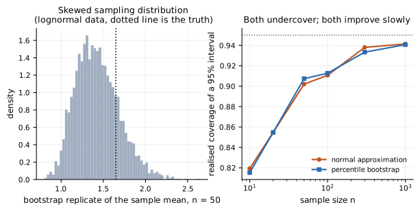
Figure 7 is a corrective to a common belief. The percentile bootstrap is not automatically better than a normal approximation; here the two are indistinguishable, because both inherit the same skewness problem. The fixes are the studentized bootstrap and the bias-corrected accelerated (BCa) interval, which adjust for skewness explicitly and are what you should use when the statistic is not roughly symmetric. The bootstrap also fails outright for non-smooth functionals: maxima, boundary parameters, and the number of distinct values are the standard counterexamples, and $m$-out-of-$n$ or subsampling is the repair.

Permutation tests give exact finite-sample validity under the sharp null of exchangeability, with no distributional assumption at all. To compare two systems on the same examples, shuffle which system produced which output within each example, recompute the metric difference many times, and read the $p$-value off the resulting distribution. This is the correct test for most NLP system comparisons and it is cheap.

Cross-validation is resampling for risk estimation rather than uncertainty. $K$-fold estimates expected test error, but its variance has no unbiased estimator (Bengio and Grandvalet, 2004), so the standard error printed next to a CV mean is optimistic. Nested cross-validation is required whenever hyperparameters are tuned inside the loop, and skipping it is one of the most common sources of inflated results in applied papers.

Stochastic approximation: SGD is an estimator

Robbins and Monro (1951) solved $E[g(\theta, X)] = 0$ with noisy evaluations, under $\sum_t \eta_t = \infty$ and $\sum_t \eta_t^2 \lt \infty$. Every optimizer in deep learning is a descendant.

The minibatch gradient is an unbiased estimate of the full gradient with covariance $\Sigma(\theta)/|B|$, so the update is a drift plus noise. In continuous time this is the SDE $d\theta = -\nabla L(\theta)\,dt + \sqrt{\eta\,\Sigma(\theta)}\,dW$, where the noise scale is set by $\eta/|B|$. Two operational consequences follow. First, the linear scaling rule: doubling the batch and doubling the learning rate leaves the noise scale unchanged, which is why Goyal and coauthors (2017) could train ImageNet in an hour, and why it breaks down past a critical batch size where the gradient is already well estimated (McCandlish, Kaplan, Amodei and the OpenAI Dota team, 2018). Second, decaying the learning rate and increasing the batch size are near-equivalent (Smith, Kindermans, Ying and Le, 2018).

The stationary distribution of that SDE is not the posterior unless you add the right noise, which is exactly what SGLD does. Treating SGD's implicit noise as Bayesian inference is a metaphor, not a theorem, and the difference shows up in every honest comparison of SGD ensembles against real posteriors.

Adam (Kingma and Ba, 2014) rescales by an estimate of the second moment, which makes it a diagonal preconditioner with a bias-correction term; the second moment estimate is a variance estimate, and the algorithm is doing crude Fisher-style normalization. Polyak-Ruppert averaging, which averages iterates rather than gradients, achieves the optimal asymptotic rate and is the theoretical ancestor of EMA weight averaging.

Part III. Information

Entropy, cross entropy, and the two KLs

Shannon entropy $H(p) = -\sum_x p(x)\log p(x)$ is the expected code length under an optimal code for $p$. Cross entropy is the length when you use a code built for $q$:

Since $H(p)$ is fixed, minimizing cross entropy is minimizing $D_{\mathrm{KL}}(p_{\text{data}}\,\|\,p_\theta)$, which is maximum likelihood. Perplexity is $\exp$ of mean negative log likelihood per token, so it is exponentiated cross entropy; bits per byte is the same in base two normalized by bytes, which is the only version comparable across tokenizers.

KL is not symmetric and the asymmetry decides what a misspecified model looks like.

Forward KL, which maximum likelihood minimizes, is infinite wherever $p$ has mass and $q$ has none, so the fit must cover everything. Reverse KL, which the ELBO minimizes, is infinite wherever $q$ has mass and $p$ has none, so the fit retreats to well-supported regions.

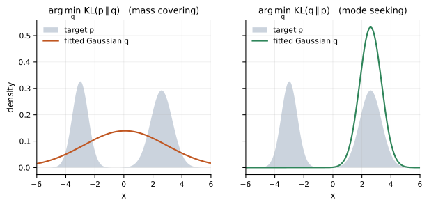
Neither is wrong; they answer different questions. Underestimated posterior variance in variational inference is this property rather than a bug, mode collapse in adversarial training is the same phenomenon, and the KL penalty in RLHF is deliberately the reverse direction because the point is to keep the policy inside the support of the reference model.

Mutual information $I(X;Y) = D_{\mathrm{KL}}(p_{XY}\,\|\,p_Xp_Y)$ obeys the data processing inequality: no function of $Y$ can increase information about $X$. Its estimation deserves suspicion. McAllester and Stratos (AISTATS 2020) proved that any distribution-free high-confidence lower bound on mutual information from $N$ samples is at most $O(\log N)$, so a contrastive objective reporting 20 nats from a batch of 256 is reporting a number no finite sample could justify. Poole and coauthors (ICML 2019) give the corresponding variance analysis of the standard variational bounds. InfoNCE is bounded above by $\log(\text{batch size})$ for exactly this reason, which is why contrastive learning benefits from large batches in a way that has nothing to do with optimization.

Fano's inequality runs the other way, lower-bounding error probability by conditional entropy, and it is how minimax lower bounds in statistics get proved.

Beyond KL: f-divergences, total variation, Wasserstein

KL belongs to the $f$-divergence family, $D_f(p\|q) = \int q(x) f(p(x)/q(x))dx$ for convex $f$ with $f(1)=0$. Total variation, $\delta(p,q) = \frac{1}{2}\int|p-q|$, is the one with an operational meaning: it is the maximum difference in probability assigned to any event, and therefore the maximum advantage of any classifier trying to tell the two apart. Pinsker's inequality connects them,

which is the tool that converts a KL budget into a bound on behavioural difference. It is the honest version of the intuition behind KL penalties in RLHF: a KL of 5 nats permits total variation up to 1, meaning no guarantee at all.

Jensen-Shannon is the symmetrized, bounded variant, and the original GAN objective (Goodfellow and coauthors, 2014) is a Jensen-Shannon minimization when the discriminator is optimal. Its problem is that JS is constant when supports are disjoint, so gradients vanish exactly when the generator is bad. Wasserstein distance,

respects the geometry of the space and stays informative between disjoint supports, which is what Arjovsky, Chintala and Bottou (2017) exploited. Nowozin, Cseke and Tomioka (2016) showed the whole $f$-divergence family can be turned into adversarial objectives by the same variational trick.

Rényi divergences interpolate and appear in privacy accounting; $\chi^2$ divergence upper-bounds KL and controls importance-weight variance directly, since $\operatorname{Var}_q[w] = \chi^2(p\|q)$. That last identity is the precise statement of why importance sampling fails under large shift.

Codes, compression, and minimum description length

Shannon's source coding theorem says the expected code length of any uniquely decodable code is at least $H(p)$, and arithmetic coding achieves it to within a bit. A probabilistic model therefore is a compressor: log loss in bits is literally the file size. This is not analogy. A language model with 0.8 bits per byte compresses text to a tenth of its ASCII size, and the same model run as an arithmetic coder produces exactly that file.

Minimum description length turns this into model selection. Choose the model minimizing the description length of model plus data, which trades fit against complexity without a prior in the Bayesian sense (Rissanen, 1978; Grünwald, 2007). Two-part MDL recovers BIC asymptotically; normalized maximum likelihood is the modern refinement.

The classical selection criteria are the same trade-off with different penalties: AIC $= -2\log \hat{L} + 2k$ estimates predictive risk and does not assume the true model is in the family; BIC $= -2\log \hat{L} + k\log n$ approximates the log marginal likelihood and does. They answer different questions, and citing whichever one supports your conclusion is a recognizable move. For Bayesian models fitted by MCMC, WAIC and PSIS-LOO (Vehtari, Gelman and Gabry, 2017) are the modern replacements, and they come with diagnostics that tell you when they have failed.

The bits-back argument connects all of this to variational inference: the ELBO gap is exactly the extra bits you pay for using an approximate posterior as a code, which makes VI a lossy compression scheme with a computable overhead.

Part IV. Models

Posteriors, conjugacy, and what more data does

Adding a prior to the likelihood gives the MAP estimate, $\arg\max_\theta[\log p_\theta(x) + \log p(\theta)]$, which is penalized likelihood: a Gaussian prior is $L_2$, a Laplace prior is $L_1$. A MAP estimate is not Bayesian in any useful sense, because a mode is not a distribution and is not reparameterization-invariant.

The posterior is the full object, and in conjugate families it is arithmetic.

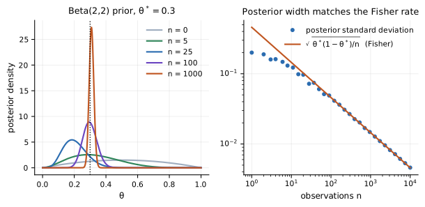
The right panel is the Bernstein-von Mises theorem in miniature: under regularity the posterior converges to a Gaussian centred at the MLE with covariance $I(\theta^*)^{-1}/n$, and the prior stops mattering. That is why Bayesian and frequentist intervals agree asymptotically for well-specified parametric models, and why the agreement fails for neural networks, where the conditions do not hold, the likelihood is not identifiable, and the posterior is neither unimodal nor concentrating in any usable sense.

Hierarchical models are the practical payoff of being Bayesian. Partial pooling across groups, $\theta_g \sim \mathcal{N}(\mu, \tau^2)$ with $\mu, \tau$ themselves estimated, produces shrinkage automatically and by the amount the data supports. That is James-Stein arrived at from the other direction, and it is the correct way to handle per-task or per-language performance estimates, which are routinely reported as independent point estimates when the sample per group is tiny.

Graphical models and conditional independence

A joint distribution over $d$ variables needs exponentially many numbers unless it factorizes, and conditional independence is what makes it factorize.

A directed model (Bayesian network) writes $p(x) = \prod_i p(x_i \mid \mathrm{pa}(x_i))$ over a DAG, and d-separation reads conditional independence off the graph. The one rule that trips everybody: conditioning on a collider creates dependence. If $X \to Z \leftarrow Y$ with $X$ and $Y$ independent, then conditioning on $Z$ makes them dependent. Selection effects, Berkson's paradox, and a large share of spurious correlations in observational data are this diagram.

An undirected model (Markov random field) writes $p(x) \propto \prod_c \psi_c(x_c)$ over cliques, with separation in the graph giving conditional independence directly (Hammersley-Clifford). The partition function is the price, and it is why energy-based models are hard to train.

Exact inference by variable elimination or the junction tree algorithm is exponential in treewidth. Belief propagation is exact on trees and a widely used approximation otherwise, and loopy BP is a fixed point of the Bethe free energy, which links it back to variational inference. The specializations are the ones most people meet first: forward-backward and Viterbi for HMMs, the Kalman filter and RTS smoother for linear-Gaussian state space models, and particle filters when neither linearity nor discreteness holds.

Attention, incidentally, is not a graphical model, but the analogy is worth stating precisely: attention weights are a data-dependent soft adjacency, not a conditional independence structure, and reading them as a probabilistic graph is a category error that has produced a lot of unreliable interpretability work.

Latent variables and EM

Mixture models, factor analysis, probabilistic PCA, topic models, and hidden Markov models are the same construction: observed $x$, unobserved $z$, and a likelihood $p(x) = \int p(x \mid z)p(z)dz$ that is intractable to maximize directly.

Expectation maximization alternates between computing the posterior over $z$ and maximizing the expected complete-data log likelihood (Dempster, Laird and Rubin, 1977). It is coordinate ascent on the same bound that variational inference maximizes, with the E step exact, and each iteration cannot decrease the likelihood.

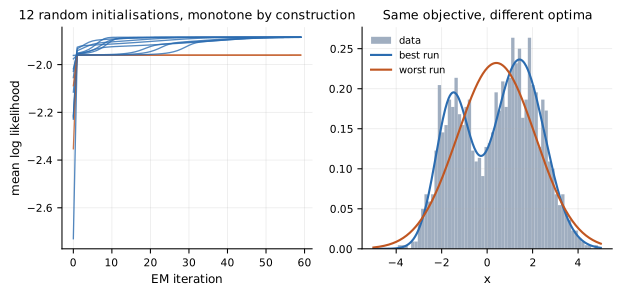
Figure 10 shows the two facts about EM that matter. Monotonicity is guaranteed and convergence to the global optimum is not, so restarts are mandatory. The likelihood surface for a Gaussian mixture with free variances is also unbounded: shrinking one component's variance onto a single point sends the likelihood to infinity, so the global maximum is a degenerate solution and what you actually want is a good local optimum or a prior that rules the singularity out.

Probabilistic PCA is the Gaussian special case, $x = Wz + \mu + \epsilon$ with isotropic noise, and its MLE recovers the principal subspace in closed form. Factor analysis relaxes the noise to diagonal. Independent component analysis replaces the Gaussian latent with a non-Gaussian one, which is what makes the solution identifiable up to permutation and scale, and Gaussianity is exactly the case where it is not. Latent Dirichlet allocation is the categorical analogue with a Dirichlet prior.

Approximate inference

Variational methods are fast and biased; MCMC is slow and asymptotically exact. Start with the identity behind all of variational inference: for any $q(z)$,

The KL term is non-negative, so $\mathcal{L}$ lower-bounds the evidence and maximizing it minimizes reverse KL to the posterior. The gap is exactly that KL, which is why an ELBO alone says nothing about posterior quality: a high ELBO and a bad posterior are entirely compatible. Mean-field factorization $q(z) = \prod_j q_j(z_j)$ makes the updates closed-form in conjugate models and systematically underestimates variance, since it cannot represent posterior correlation.

The VAE amortizes $q_\phi(z\mid x)$ with a network, adding an amortization gap on top of the approximation gap. Normalizing flows, importance-weighted bounds (IWAE), and semi-amortized schemes each close part of it.

MCMC gives up speed for correctness. Metropolis-Hastings proposes $x'$ from $q(\cdot\mid x)$ and accepts with

which satisfies detailed balance and leaves $p$ invariant while needing $p$ only up to a constant. Gibbs sampling is the special case that samples each coordinate from its full conditional and always accepts.

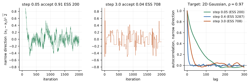
Small steps are almost always accepted and move nowhere; large steps are almost always rejected. Roberts, Gelman and Gilks (1997) showed the asymptotically optimal acceptance rate for a product target in high dimension is 0.234, achieved by scaling the proposal standard deviation as $2.38/\sqrt{d}$. Hamiltonian Monte Carlo replaces the random walk with simulated dynamics of $H(x,v) = -\log p(x) + \frac{1}{2}\|v\|^2$ under a leapfrog integrator with a Metropolis correction (Neal, 2011), and NUTS removes the trajectory-length parameter (Hoffman and Gelman, 2014). At network scale, stochastic gradient Langevin dynamics adds the right amount of noise to SGD,

targeting the posterior as $\eta_t \to 0$ (Welling and Teh, 2011). Whether the samples resemble the posterior at usable step sizes is a separate question, and Izmailov and coauthors (2021) ran full-batch HMC on small networks to check: cheap approximations differ from the real posterior in ways that change conclusions.

Diagnostics are not optional. Run several chains from dispersed starts, compute $\hat R$ (the rank-normalized split version of Gelman-Rubin), and report effective sample size per parameter. A single chain that looks stationary is the most common way to publish a wrong posterior.

Generative models are probability statements

Each family makes different operations cheap. Autoregressive models factor by the chain rule and give exact likelihood with sequential sampling. Flows give exact likelihood and fast sampling at the cost of invertibility. VAEs give a bound and fast sampling. Energy-based models give unnormalized densities and need MCMC or a surrogate objective such as contrastive divergence or noise-contrastive estimation. GANs give samples and no likelihood at all. Diffusion models give a bound and slow sampling, and currently win on perceptual quality in continuous domains.

The diffusion forward process is a fixed Gaussian chain, $q(x_t\mid x_{t-1}) = \mathcal{N}(\sqrt{1-\beta_t}x_{t-1}, \beta_t I)$, with closed-form marginals. Writing $\alpha_t = 1-\beta_t$ and $\bar\alpha_t = \prod_{s\le t}\alpha_s$,

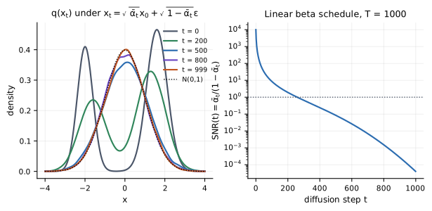
Because that marginal is Gaussian, its score is exact for known $x_0$:

Vincent (2011) proved that regressing on this conditional score matches the score of the marginal $q(x_t)$ up to a constant, which is the quantity you need and cannot compute. That identity licenses the objective of Ho, Jain and Abbeel (2020):

Predicting the noise is predicting the score. Sohl-Dickstein and coauthors (2015) set up the variational argument, Song and Ermon (2019) reached the same place from score matching (Hyvärinen, 2005), and Song and coauthors (2021) unified both as discretizations of an SDE with an associated deterministic probability-flow ODE. The reweighting between the true ELBO and the simple loss is not innocent: it trades likelihood for sample quality, which is why diffusion models report excellent samples and unremarkable bits per dimension.

Bias, variance, and the curve that breaks the story

For squared loss the expected test error decomposes exactly, with expectations over training sets:

It is a theorem for squared loss and only that; the extensions to 0-1 loss are several and inequivalent.

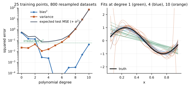
That picture is correct and incomplete. Belkin, Hsu, Ma and Mandal (PNAS 2019) and Nakkiran and coauthors (2019) documented that test error peaks where the model can just barely interpolate, then falls again.

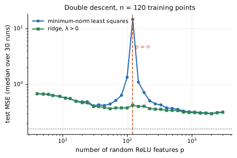
The peak is the Marchenko-Pastur fact from Part I: at $p=n$ the smallest eigenvalue of the design touches zero, so the interpolating solution has enormous norm. Past that point many interpolants exist and the minimum-norm one is well behaved. Nakkiran, Venkat, Kakade and Ma (ICLR 2021) proved optimally tuned ridge is monotone in model size for isotropic linear models, and the green curve reproduces it. Double descent is a statement about unregularized interpolation, not about overparameterization as such.

Generalization bounds

Empirical risk minimization picks $\hat h = \arg\min_{h\in\mathcal{H}} \frac{1}{n}\sum_i \ell(h(x_i),y_i)$, and because $\hat h$ depends on the data, Hoeffding does not apply and you need uniform control.

Rademacher complexity gives the cleanest form. With $\mathfrak{R}_n(\mathcal{H}) = E_{\sigma,S}\big[\sup_h \frac{1}{n}\sum_i \sigma_i h(x_i)\big]$, with probability $1-\delta$ and loss in $[0,1]$,

Bartlett and Mendelson (2002) established the line; VC dimension is the older combinatorial version, recovering $\sqrt{d/n}$ for simple classes.

Applied to neural networks these are numerically vacuous, meaning the right-hand side exceeds one and the bound asserts less than random guessing. Zhang, Bengio, Hardt, Recht and Vinyals (ICLR 2017) made the point unavoidable by fitting CIFAR-10 with random labels to zero training error, which forces any capacity bound on that architecture to be trivial.

PAC-Bayes is the framework that has produced non-vacuous numbers. For a prior $P$ fixed before the data and any posterior $Q$, with probability $1-\delta$,

McAllester (1999) introduced it; Dziugaite and Roy (UAI 2017) optimized $Q$ directly and got the first non-vacuous guarantee for a stochastic network with more parameters than training data. The bound rewards posteriors concentrated near the prior, a formal version of the flat-minima intuition.

Algorithmic stability gives an alternative route that bounds generalization by how much the output changes when one example is swapped, and it applies to SGD directly (Hardt, Recht and Singer, 2016). Information-theoretic bounds replace the KL term with the mutual information between the training set and the learned weights, which is appealing and usually just as hard to compute.

Scaling laws sit oddly beside all this. Kaplan and coauthors (2020) and Hoffmann and coauthors (2022) fit power laws in parameters, data and compute that predict held-out loss across orders of magnitude with no generalization theory behind them. They are regressions with confidence bands, they have been far more useful for planning than any bound in this section, and treating them as laws rather than fits is the error to avoid.

Part V. Sequential decisions

Markov chains and stochastic processes

A Markov chain has $p(x_{t+1}\mid x_{1:t}) = p(x_{t+1}\mid x_t)$. An irreducible aperiodic chain on a finite space has a unique stationary distribution $\pi = \pi P$ and converges to it geometrically, at a rate governed by the spectral gap $1-|\lambda_2|$. Detailed balance, $\pi(x)P(x\to y) = \pi(y)P(y\to x)$, is a sufficient condition for stationarity and is what Metropolis-Hastings constructs by hand. Mixing time is the number of steps to get within total variation $\epsilon$ of $\pi$, and it is the honest measure of MCMC cost; effective sample size is its empirical proxy.

Beyond chains, three processes recur. The Poisson process models event arrivals with independent increments and exponential gaps, and its intensity function is what survival and hazard models estimate. Brownian motion is the continuous limit of a random walk, and the SDE $dx = b(x)dt + \sigma(x)dW$ with its Fokker-Planck equation for the evolving density is the language diffusion models and SGD analyses share. Martingales, $E[X_{t+1}\mid \mathcal{F}_t] = X_t$, give the optional stopping theorem and Azuma-Hoeffding, which is how you get concentration for adaptively collected data, and it is the technical core of both bandit analysis and anytime-valid inference.

Gaussian processes are the function-space object: any finite collection of function values is jointly Gaussian, prediction is the conditioning formula from Part I, and the kernel encodes the prior over functions. Cost is $O(n^3)$, which inducing-point and random-feature approximations attack. A wide neural network at initialization is a Gaussian process, and its training dynamics under gradient flow are described by the neural tangent kernel, which is the cleanest bridge between deep learning and classical nonparametrics even though it does not describe feature learning.

Bandits and the cost of exploration

The multi-armed bandit is the minimal model of learning while acting. Pull arm $a$, receive a reward from an unknown distribution, and measure regret against always pulling the best arm:

Lai and Robbins (1985) proved that any consistent algorithm has regret at least $\Omega(\log T)$ with a constant given by the KL divergence between arm distributions, so logarithmic regret is optimal and the constant is information-theoretic.

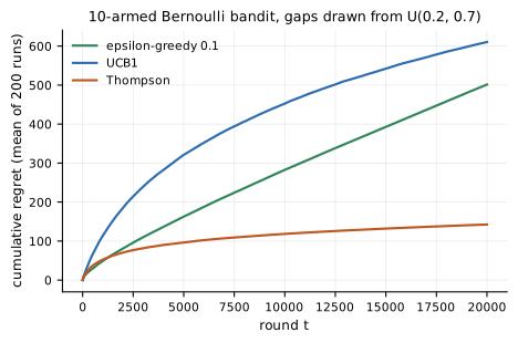
Epsilon-greedy with a constant rate has linear regret, visible as the straight line: it keeps paying to explore forever. UCB1 picks $\arg\max_a \hat\mu_a + \sqrt{2\log t / n_a}$, an upper confidence bound derived from Hoeffding, and achieves logarithmic regret with a conservative constant, which is why it is beaten here by Thompson sampling. Thompson sampling (1933) draws a parameter from the posterior of each arm and acts greedily on the draw, which is Bayesian, trivially implementable for conjugate rewards, and has matching optimal regret bounds (Agrawal and Goyal, 2012; Russo and Van Roy). Its practical dominance in this figure is typical rather than an artifact.

The structure carries directly into machine learning practice. Hyperparameter search is a bandit, A/B testing with early stopping is a bandit, and best-arm identification (pure exploration, where regret during learning does not count) is the right formalization of model selection and needs different algorithms from regret minimization. Contextual bandits add features and are the standard model for recommendation, where logged data creates the same off-policy evaluation problem the next section discusses.

Reinforcement learning as probability

A Markov decision process is a chain with actions and rewards, and the value function is a conditional expectation:

The Bellman equation is the law of total expectation applied recursively, and temporal-difference learning is stochastic approximation applied to it: the TD error is an unbiased sample of the residual, and Robbins-Monro conditions give convergence in the tabular case.

Policy gradients are the score-function estimator from Part II with the trajectory distribution as $q_\theta$:

where the advantage is the baseline-subtracted return, and the baseline is variance reduction and nothing else. Everything else in the modern recipe is variance control: GAE trades bias for variance in the advantage estimate, and PPO's clipped ratio is a trust region on the importance weight $\pi_\theta/\pi_{\text{old}}$, which is the same weight-degeneracy problem from Figure 4 in a different costume.

Off-policy evaluation is importance sampling with the same failure mode, and it is worse in sequential settings because the weight is a product over timesteps, so its variance grows exponentially in horizon. Doubly robust estimators combine a model-based estimate with an importance-weighted correction and are unbiased if either component is right.

RLHF is this machinery with a learned reward. Preferences are usually modelled with Bradley-Terry (1952):

so reward-model training is logistic regression on pairwise comparisons, and the reward is identified only up to an additive constant per prompt. The KL penalty against a reference policy is a reverse-KL trust region, and Gao, Schulman and Hilton (2022) measured the overoptimization curve: as the policy moves away from the reference, proxy reward keeps rising while true reward turns over, with the gap growing roughly in $\sqrt{D_{\mathrm{KL}}}$. That is a statistical statement about a fitted reward model being an estimate with error, not a claim about alignment in general.

Causal inference

Prediction and intervention are different questions and no amount of predictive accuracy converts one into the other. The distinction is $p(y \mid x)$ against $p(y \mid do(x))$, and they differ whenever a confounder causes both.

Two formalisms, largely interchangeable. Potential outcomes (Neyman, Rubin) writes $Y_i(1)$ and $Y_i(0)$ for what would happen to unit $i$ under each treatment, notes that only one is observed, and defines the average treatment effect as $E[Y(1)-Y(0)]$. Structural causal models (Pearl) write the system as assignments $X_i = f_i(\mathrm{pa}_i, U_i)$ over a DAG, and define intervention as deleting the assignment for $X$ and setting it.

Identification is the whole game. Randomization makes treatment independent of potential outcomes, so the difference in means is unbiased, which is why an RCT is the reference standard. Without randomization you need an assumption, and the assumption is not testable from the data. The backdoor criterion says adjusting for a set $Z$ blocking all backdoor paths identifies the effect; the frontdoor criterion works through a fully mediating variable; instrumental variables use a source of variation affecting treatment only through the outcome path. Propensity score methods implement backdoor adjustment by modelling $p(\text{treatment}\mid Z)$, and inverse propensity weighting is importance sampling again, with the same variance blowup when propensities approach zero or one.

Two traps worth naming. Conditioning on a collider or on a post-treatment variable creates bias rather than removing it, so "control for everything available" is wrong advice. And Simpson's paradox is not a curiosity: an association can reverse in every subgroup relative to the aggregate, and which analysis is correct depends entirely on the causal graph, not on the data.

Machine learning connections are direct. Covariate shift correction is a causal-style reweighting; off-policy evaluation is causal effect estimation with a known propensity, which is the easy case; double machine learning (Chernozhukov and coauthors) uses flexible models for nuisance functions with cross-fitting to preserve valid inference on the effect; and the reason A/B tests remain necessary despite excellent predictive models is that no observational metric identifies the interventional quantity you care about.

Part VI. Measurement

Calibration and proper scoring rules

A classifier is calibrated if among cases assigned probability 0.7 it is right 70% of the time. Accuracy says nothing about this, and the first requirement for measuring it is a scoring rule that cannot be gamed.

A scoring rule is proper if the expected score is optimized by reporting the true distribution, strictly proper if uniquely so. Log loss and Brier are strictly proper; accuracy, F1 and AUC are not, which is why a model can improve on them by becoming more confident without becoming more correct. Gneiting and Raftery (2007) is the reference; Allan Murphy's 1973 partition splits Brier into reliability, resolution and uncertainty, separating "are the probabilities right" from "do they discriminate".

Expected calibration error bins by confidence and averages the gap,

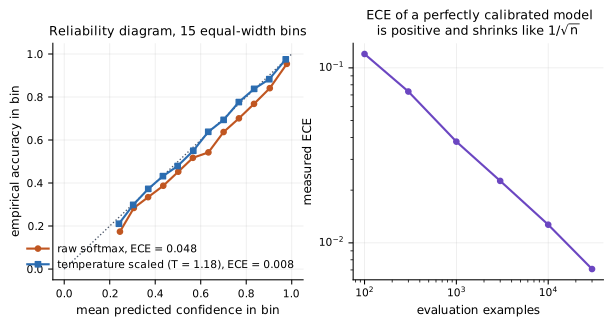
The right panel is the part that gets forgotten. ECE takes an absolute value inside the bin average, so sampling noise cannot cancel and the estimator is biased upward. Comparing the ECE of two models evaluated on differently sized sets, or with different bin counts, compares mostly estimation noise. Report log loss alongside it and treat small ECE differences as unmeasured.

Temperature scaling divides logits by one scalar fitted by minimizing validation NLL, leaving the argmax and therefore accuracy untouched. Guo, Pleiss, Sun and Weinberger (2017) showed it removes most of the miscalibration of modern image classifiers; the synthetic example above needed $T = 1.18$. Isotonic regression and Platt scaling are the nonparametric and binary alternatives.

Separating the two sources of uncertainty is worth the effort. Aleatoric uncertainty is noise in the data-generating process and does not shrink with more data; epistemic uncertainty is parameter ignorance and does. Deep ensembles (Lakshminarayanan, Pritzel and Blundell, 2017) remain a strong baseline for the epistemic part, MC dropout (Gal and Ghahramani, 2016) is the cheap approximation, and Ovadia and coauthors (2019) found every method degrades badly under distribution shift.

Coverage without assumptions

Conformal prediction gives finite-sample coverage with no model assumption and only exchangeability. Split conformal: compute nonconformity scores $s_i$ on a calibration set of size $n$, take

and predict $C(x) = \{y : s(x,y)\le \hat q\}$. Then $P(Y_{n+1}\in C(X_{n+1})) \ge 1-\alpha$, with an upper bound of $1-\alpha+1/(n+1)$. The ceiling correction is not decoration: the ordinary empirical quantile undercovers.

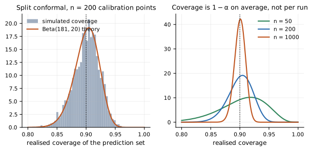
The guarantee is marginal in two senses, and Figure 17 shows the first. Coverage is $1-\alpha$ averaged over calibration sets, so a deployed model has a realised coverage drawn from a Beta distribution; with 50 calibration points an 85% realised rate for a nominal 90% procedure is unremarkable. Coverage is also marginal over $x$, so a set can hit 90% overall while covering one subgroup 99% of the time and another 60%. Mondrian and group-conditional variants address the second; nothing addresses the first except more calibration data. Vovk, Gammerman and Shafer (2005) is the source, Angelopoulos and Bates (2021) the readable introduction, and Barber, Candes, Ramdas and Tibshirani (2023) work out what survives when exchangeability fails.

Discrimination metrics, and what imbalance does to them

ROC curves plot true positive rate against false positive rate, and AUC is the probability that a random positive scores above a random negative. Both are invariant to class prevalence, which is sometimes the point and often the problem.

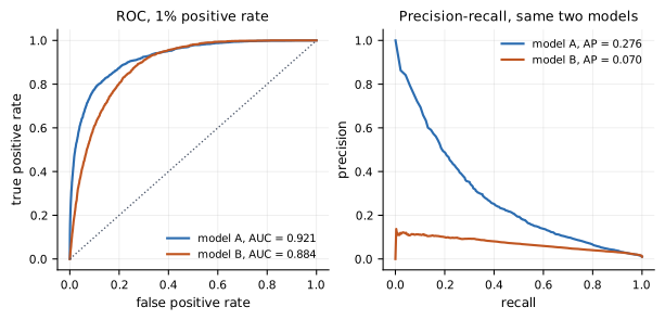
The reason is that a false positive rate of 0.1 at a 1% base rate means ten false positives for every true one, and the ROC axis makes that invisible. Precision depends on prevalence and is what an operator actually experiences. When positives are rare, report precision-recall, average precision, or precision at a fixed recall, and state the base rate. AUC is the right summary when you need a prevalence-invariant ranking quality and the wrong one when you are deciding whether a system is deployable.

The same arithmetic drives the fairness impossibility results. Chouldechova (2017) and Kleinberg, Mullainathan and Raghavan (2016) proved that calibration within groups, equal false positive rates, and equal false negative rates cannot all hold simultaneously when base rates differ across groups, except in degenerate cases. That is a theorem about confusion matrices, not a political claim, and it means a fairness criterion has to be chosen rather than satisfied in general.

Distribution shift

Training and deployment distributions differ, and the flavour determines the fix. Covariate shift changes $p(x)$ with $p(y\mid x)$ fixed; label shift changes $p(y)$ with $p(x\mid y)$ fixed; concept drift changes $p(y\mid x)$ itself and no reweighting can repair it.

Under covariate shift the target risk is estimable by importance weighting, $E_{p_{\text{te}}}[\ell] = E_{p_{\text{tr}}}[w(x)\ell]$ with $w = p_{\text{te}}/p_{\text{tr}}$, which is Part II's machinery again with the same failure mode.

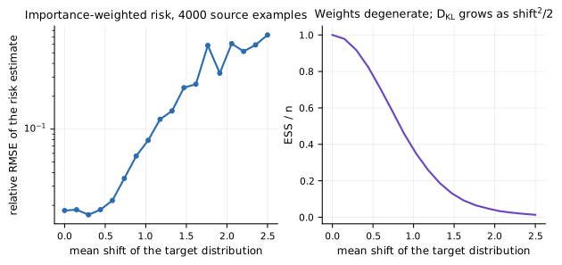
The KL divergence between the two Gaussians here grows as shift squared over two, and the weight variance grows exponentially in that, which is the $\chi^2$ identity from Part III. Practically: importance weighting works for mild shift and silently fails for severe shift, and ESS is the diagnostic that tells you which regime you are in. Label shift is the easier case, where BBSE and its relatives estimate the target label distribution from a confusion matrix and reweight consistently. For detection rather than correction, two-sample tests on model outputs or embeddings (MMD, classifier two-sample tests) are the standard tools, and univariate tests on raw features are near-useless in high dimension for the reasons in Part I.

Hypothesis testing and benchmark claims

This is where the field is weakest and the weakness is fixable.

The Neyman-Pearson framework fixes a null, a test statistic, and a rejection region with Type I error $\alpha$; power is one minus Type II error and depends on the effect size, the variance, and $n$. A $p$-value is the probability of a statistic at least this extreme under the null, and it is not the probability the null is true, nor the probability the result replicates. The likelihood ratio test with Wilks' theorem gives the asymptotic $\chi^2$ reference for nested models.

A reported accuracy carries at least three variance sources: the finite test set, the seed (initialization, data order, augmentation), and the hyperparameter search. Bouthillier and fifteen coauthors (MLSys 2021) measured all three across five tasks and found seed and hyperparameter variance comparable to test-set variance rather than negligible beside it. They also report that an estimator randomizing over more sources approximates the ideal comparison better, at a 51-fold reduction in compute, than one that fixes everything and varies only the test set.

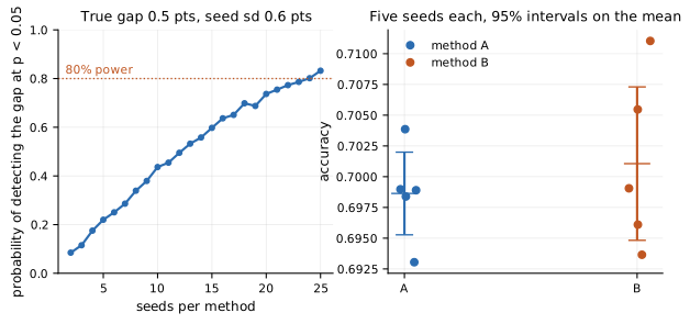
Figure 20 explains a familiar experience. Most published improvements sit where a five-seed experiment has roughly a one-in-five chance of finding a real effect, which also means the effects that clear the bar are systematically overestimated: the winner's curse is arithmetic, not sociology.

Four practices, in rough order of payoff. Pair the comparison, evaluating both systems on the same examples and testing per-example differences with a paired bootstrap, a permutation test, or McNemar's test for binary correctness; pairing removes example difficulty from the variance and is usually worth more than doubling the test set. Report a distribution over seeds rather than a maximum, since a max is an estimate of the upper tail that improves with compute spent. Bootstrap the metric of interest directly when no closed-form standard error exists. And correct for multiplicity in tables: twenty comparisons at the 5% level produce a false positive by construction, and Benjamini-Hochberg (1995) controls the false discovery rate at far less cost than Bonferroni.

For comparisons across many datasets, Demšar (2006) recommends the Friedman test with post-hoc pairwise procedures rather than averaging accuracies across tasks, which is not a meaningful operation. Dietterich (1998) worked out which resampling schemes have acceptable Type I error for classifier comparison, and repeated random splits with a naive $t$-test is not among them.

One newer tool deserves adoption. Peeking at a fixed-$\alpha$ test invalidates it, which is why continuous monitoring of an A/B test inflates error rates. E-values and confidence sequences give anytime-valid inference: you may stop whenever you like and the guarantee holds, at the price of a modest constant (Ramdas, Grünwald, Vovk and Shafer, 2023). For online evaluation and for expensive training runs you might want to abort, this is the correct framework rather than a workaround.

Statistics specific to language models

Decoding is repeated sampling from a categorical distribution that has been deliberately distorted. Temperature rescales logits, $p_i \propto \exp(z_i/T)$, a monotone transformation that changes spread without changing order. Top-$k$ truncates to the $k$ most likely tokens; nucleus sampling truncates to the smallest set exceeding mass $p$ (Holtzman, Buys, Du, Forbes and Choi, 2019), adapting the cutoff to how peaked the position is.

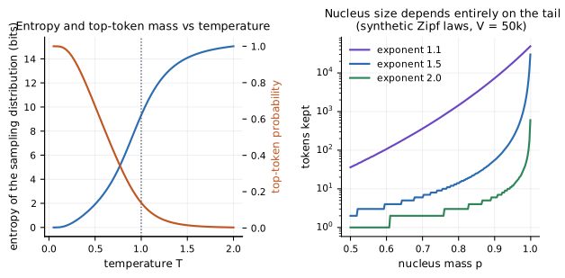
Nucleus size is determined entirely by the tail, so the same $p = 0.9$ can mean six candidates or seven thousand. Reporting decoding hyperparameters without the entropy they induce says very little, and comparing a $p$ value across models is comparing two different truncations.

Evaluation has its own estimators, and one of them is routinely got wrong. For pass@$k$, drawing $n \ge k$ samples per problem and counting $c$ correct, the unbiased estimator is

as used by Chen and coauthors (2021). The plug-in alternative $1-(1-c/n)^k$ is biased downward, badly.

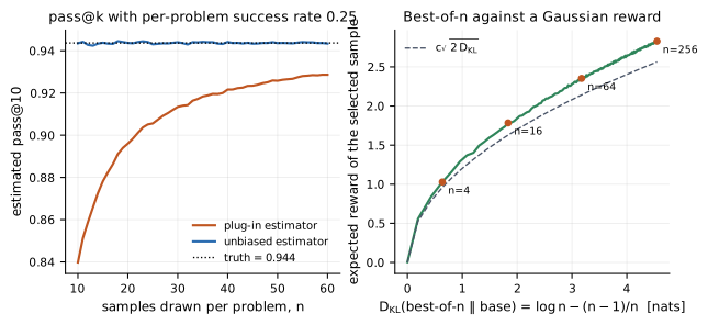
A ten-point bias on a headline metric is not a rounding issue, and it comes from applying an estimator to a nonlinear function of a rate. The right panel is the other identity worth knowing: best-of-$n$ sampling induces a policy whose KL divergence from the base is exactly $\log n - (n-1)/n$, so $n=16$ costs 1.84 nats and $n=256$ costs 4.55. Reward rises roughly as the square root of KL, which is the same shape Gao, Schulman and Hilton (2022) fitted for RLHF overoptimization, and it means best-of-$n$ and RL fine-tuning can be compared on a common axis rather than by vibes.

Three more measurement issues specific to this setting. Contamination: a benchmark that entered pretraining breaks exchangeability between test and deployment, and the standard detections (n-gram overlap, canary strings, membership tests) all have low power, so absence of evidence is weak here. LLM-as-judge: a judge is a measurement instrument with its own bias and variance, exhibits position and verbosity effects, and its agreement with humans should be reported as a calibration statistic rather than assumed (Zheng and coauthors, 2023). And multiple-choice scoring: length normalization, answer-order permutation, and the choice between scoring the letter and scoring the option text change rankings, so any comparison should fix the protocol and report it.

Kadavath and coauthors (2022) found language models assign reasonably calibrated probabilities to the correctness of their own answers in multiple-choice format, which makes the token distribution a usable uncertainty signal. Any post-hoc distortion of that distribution destroys the calibration, so a sampler tuned for text quality and a probability read off for confidence are in direct conflict.

Differential privacy

Privacy is a probabilistic guarantee about an algorithm, not a property of data. A randomized mechanism $M$ is $(\epsilon,\delta)$-differentially private if for all adjacent datasets $D, D'$ differing in one record and all measurable $S$,

The Gaussian mechanism achieves it by adding noise with $\sigma \ge \Delta_2\sqrt{2\ln(1.25/\delta)}/\epsilon$, where $\Delta_2$ is the $L_2$ sensitivity of the query.

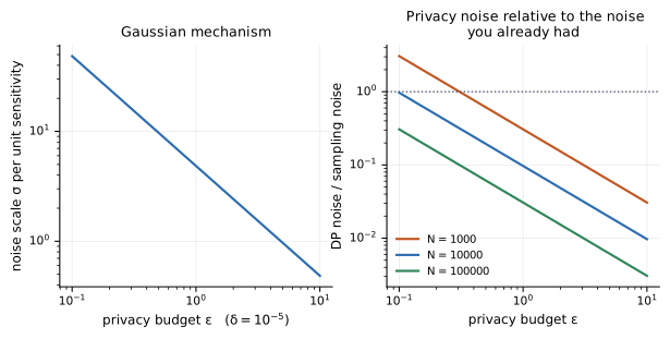
The right panel is the argument that makes DP practical for aggregate statistics: privacy noise scales as $1/(N\epsilon)$ while sampling noise scales as $1/\sqrt{N}$, so for large $N$ the privacy cost is dominated by noise you already had. The reason DP-SGD is nonetheless expensive is that training queries the data thousands of times, and composition accumulates. Basic composition adds $\epsilon$ linearly; advanced composition gives $\sqrt{k}$ growth; the moments accountant and Rényi DP give much tighter bounds and are what makes DP-SGD feasible at all (Abadi and coauthors, 2016). Per-example gradient clipping sets the sensitivity, and it is also a bias: clipping changes the expected gradient direction, so DP-SGD optimizes a slightly different objective than SGD.

Membership inference is the attack DP defends against, and it is a hypothesis test: given a model and a record, decide whether the record was in training. Framing it that way makes the connection exact, since $\epsilon$ bounds the achievable ROC of any such test.

Identities worth keeping in working memory

Everything above reduces to a small set of manipulations. In rough order of how often I reach for them:

Five of the nine are statements about changing the distribution you integrate against. That is not a coincidence, and it is the practical thesis of this piece: most of the failures I have watched were failures to notice the distribution had changed. A proposal that stopped covering its target. An evaluation set no longer exchangeable with deployment. A calibration split reused for model selection. A benchmark that entered the pretraining corpus. A policy that drifted far enough from its reference that the reward model was extrapolating. The mathematics in each case was settled decades ago; the habit of asking which distribution you are under, at every step, is the part that has to be practised.

References

Foundations, probability and high-dimensional statistics

• Billingsley, P. (1995). Probability and Measure, 3rd ed. Wiley.
• Boucheron, S., Lugosi, G. and Massart, P. (2013). Concentration Inequalities. Oxford University Press.
• Casella, G. and Berger, R. L. (2002). Statistical Inference, 2nd ed. Duxbury.
• Efron, B. and Hastie, T. (2016). Computer Age Statistical Inference. Cambridge University Press.
• Hoeffding, W. (1963). Probability inequalities for sums of bounded random variables. JASA 58(301), 13-30.
• van der Vaart, A. W. (1998). Asymptotic Statistics. Cambridge University Press.
• Vershynin, R. (2018). High-Dimensional Probability. Cambridge University Press.
• Wainwright, M. J. (2019). High-Dimensional Statistics: A Non-Asymptotic Viewpoint. Cambridge University Press.

Machine learning texts

• Bishop, C. M. (2006). Pattern Recognition and Machine Learning. Springer.
• Cover, T. M. and Thomas, J. A. (2006). Elements of Information Theory, 2nd ed. Wiley.
• Gelman, A., Carlin, J. B., Stern, H. S., Dunson, D. B., Vehtari, A. and Rubin, D. B. (2013). Bayesian Data Analysis, 3rd ed. CRC Press.
• Koller, D. and Friedman, N. (2009). Probabilistic Graphical Models. MIT Press.
• Lattimore, T. and Szepesvári, C. (2020). Bandit Algorithms. Cambridge University Press.
• Murphy, K. P. (2022, 2023). Probabilistic Machine Learning: An Introduction and Advanced Topics. MIT Press.
• Rasmussen, C. E. and Williams, C. K. I. (2006). Gaussian Processes for Machine Learning. MIT Press.
• Sutton, R. S. and Barto, A. G. (2018). Reinforcement Learning: An Introduction, 2nd ed. MIT Press.
• Wainwright, M. J. and Jordan, M. I. (2008). Graphical models, exponential families, and variational inference. Foundations and Trends in Machine Learning 1(1-2).

Estimation, optimization and inference

• Amari, S. (1998). Natural gradient works efficiently in learning. Neural Computation 10(2), 251-276.
• Bengio, Y. and Grandvalet, Y. (2004). No unbiased estimator of the variance of K-fold cross-validation. JMLR 5, 1089-1105.
• Blei, D. M., Kucukelbir, A. and McAuliffe, J. D. (2017). Variational inference: a review for statisticians. JASA 112(518). arXiv:1601.00670
• Dempster, A. P., Laird, N. M. and Rubin, D. B. (1977). Maximum likelihood from incomplete data via the EM algorithm. JRSS-B 39(1), 1-38.
• Efron, B. (1979). Bootstrap methods: another look at the jackknife. Annals of Statistics 7(1), 1-26.
• Goyal, P. et al. (2017). Accurate, large minibatch SGD: training ImageNet in 1 hour. arXiv:1706.02677
• Hoffman, M. D. and Gelman, A. (2014). The No-U-Turn sampler. JMLR 15, 1593-1623.
• Izmailov, P., Vikram, S., Hoffman, M. D. and Wilson, A. G. (2021). What are Bayesian neural network posteriors really like? ICML. arXiv:2104.14421
• James, W. and Stein, C. (1961). Estimation with quadratic loss. Berkeley Symposium on Mathematical Statistics and Probability.
• Jang, E., Gu, S. and Poole, B. (2016). Categorical reparameterization with Gumbel-softmax. arXiv:1611.01144
• Kingma, D. P. and Ba, J. (2014). Adam: a method for stochastic optimization. arXiv:1412.6980
• Kingma, D. P. and Welling, M. (2013). Auto-encoding variational Bayes. arXiv:1312.6114
• Maddison, C. J., Mnih, A. and Teh, Y. W. (2016). The concrete distribution. arXiv:1611.00712
• McCandlish, S., Kaplan, J., Amodei, D. et al. (2018). An empirical model of large-batch training. arXiv:1812.06162
• Neal, R. M. (2011). MCMC using Hamiltonian dynamics. In Handbook of Markov Chain Monte Carlo.
• Rezende, D. J., Mohamed, S. and Wierstra, D. (2014). Stochastic backpropagation and approximate inference in deep generative models. arXiv:1401.4082
• Robbins, H. and Monro, S. (1951). A stochastic approximation method. Annals of Mathematical Statistics 22(3), 400-407.
• Roberts, G. O., Gelman, A. and Gilks, W. R. (1997). Weak convergence and optimal scaling of random walk Metropolis algorithms. Annals of Applied Probability 7(1), 110-120.
• Smith, S. L., Kindermans, P.-J., Ying, C. and Le, Q. V. (2018). Don't decay the learning rate, increase the batch size. ICLR. arXiv:1711.00489
• Welling, M. and Teh, Y. W. (2011). Bayesian learning via stochastic gradient Langevin dynamics. ICML.
• Williams, R. J. (1992). Simple statistical gradient-following algorithms for connectionist reinforcement learning. Machine Learning 8, 229-256.

Information theory and model selection

• Grünwald, P. D. (2007). The Minimum Description Length Principle. MIT Press.
• McAllester, D. and Stratos, K. (2020). Formal limitations on the measurement of mutual information. AISTATS, PMLR 108, 875-884. arXiv:1811.04251
• Poole, B., Ozair, S., van den Oord, A., Alemi, A. A. and Tucker, G. (2019). On variational bounds of mutual information. ICML, PMLR 97, 5171-5180.
• Rissanen, J. (1978). Modeling by shortest data description. Automatica 14(5), 465-471.
• Vehtari, A., Gelman, A. and Gabry, J. (2017). Practical Bayesian model evaluation using leave-one-out cross-validation and WAIC. Statistics and Computing 27, 1413-1432. arXiv:1507.04544

Generalization

• Bartlett, P. L. and Mendelson, S. (2002). Rademacher and Gaussian complexities. JMLR 3, 463-482.
• Belkin, M., Hsu, D., Ma, S. and Mandal, S. (2019). Reconciling modern machine-learning practice and the classical bias-variance trade-off. PNAS 116(32), 15849-15854.
• Dziugaite, G. K. and Roy, D. M. (2017). Computing nonvacuous generalization bounds for deep (stochastic) neural networks with many more parameters than training data. UAI. arXiv:1703.11008
• Hardt, M., Recht, B. and Singer, Y. (2016). Train faster, generalize better: stability of stochastic gradient descent. ICML.
• Hoffmann, J. et al. (2022). Training compute-optimal large language models. arXiv:2203.15556
• Kaplan, J. et al. (2020). Scaling laws for neural language models. arXiv:2001.08361
• McAllester, D. A. (1999). PAC-Bayesian model averaging. COLT.
• Nakkiran, P., Kaplun, G., Bansal, Y., Yang, T., Barak, B. and Sutskever, I. (2019). Deep double descent. arXiv:1912.02292
• Nakkiran, P., Venkat, P., Kakade, S. and Ma, T. (2021). Optimal regularization can mitigate double descent. ICLR. arXiv:2003.01897
• Zhang, C., Bengio, S., Hardt, M., Recht, B. and Vinyals, O. (2017). Understanding deep learning requires rethinking generalization. ICLR. arXiv:1611.03530

Generative models

• Arjovsky, M., Chintala, S. and Bottou, L. (2017). Wasserstein GAN. arXiv:1701.07875
• Goodfellow, I. et al. (2014). Generative adversarial networks. arXiv:1406.2661
• Ho, J., Jain, A. and Abbeel, P. (2020). Denoising diffusion probabilistic models. arXiv:2006.11239
• Hyvärinen, A. (2005). Estimation of non-normalized statistical models by score matching. JMLR 6, 695-709.
• Nowozin, S., Cseke, B. and Tomioka, R. (2016). f-GAN. arXiv:1606.00709
• Papamakarios, G., Nalisnick, E., Rezende, D. J., Mohamed, S. and Lakshminarayanan, B. (2021). Normalizing flows for probabilistic modeling and inference. JMLR 22. arXiv:1912.02762
• Rezende, D. J. and Mohamed, S. (2015). Variational inference with normalizing flows. arXiv:1505.05770
• Sohl-Dickstein, J., Weiss, E. A., Maheswaranathan, N. and Ganguli, S. (2015). Deep unsupervised learning using nonequilibrium thermodynamics. arXiv:1503.03585
• Song, Y. and Ermon, S. (2019). Generative modeling by estimating gradients of the data distribution. arXiv:1907.05600
• Song, Y., Sohl-Dickstein, J., Kingma, D. P., Kumar, A., Ermon, S. and Poole, B. (2021). Score-based generative modeling through stochastic differential equations. ICLR. arXiv:2011.13456
• van den Oord, A., Li, Y. and Vinyals, O. (2018). Representation learning with contrastive predictive coding. arXiv:1807.03748
• Vincent, P. (2011). A connection between score matching and denoising autoencoders. Neural Computation 23(7), 1661-1674.

Sequential decisions and causality

• Agrawal, S. and Goyal, N. (2012). Analysis of Thompson sampling for the multi-armed bandit problem. COLT.
• Auer, P., Cesa-Bianchi, N. and Fischer, P. (2002). Finite-time analysis of the multiarmed bandit problem. Machine Learning 47, 235-256.
• Bradley, R. A. and Terry, M. E. (1952). Rank analysis of incomplete block designs. Biometrika 39(3/4), 324-345.
• Gao, L., Schulman, J. and Hilton, J. (2022). Scaling laws for reward model overoptimization. arXiv:2210.10760
• Imbens, G. W. and Rubin, D. B. (2015). Causal Inference for Statistics, Social, and Biomedical Sciences. Cambridge University Press.
• Lai, T. L. and Robbins, H. (1985). Asymptotically efficient adaptive allocation rules. Advances in Applied Mathematics 6(1), 4-22.
• Pearl, J. (2009). Causality, 2nd ed. Cambridge University Press.
• Thompson, W. R. (1933). On the likelihood that one unknown probability exceeds another. Biometrika 25(3/4), 285-294.

Uncertainty, evaluation and privacy

• Abadi, M. et al. (2016). Deep learning with differential privacy. CCS. arXiv:1607.00133
• Angelopoulos, A. N. and Bates, S. (2021). A gentle introduction to conformal prediction and distribution-free uncertainty quantification. arXiv:2107.07511. Expanded as Foundations and Trends in Machine Learning 16(4), 494-591.
• Barber, R. F., Candes, E. J., Ramdas, A. and Tibshirani, R. J. (2023). Conformal prediction beyond exchangeability. Annals of Statistics 51(2), 816-845.
• Benjamini, Y. and Hochberg, Y. (1995). Controlling the false discovery rate. JRSS-B 57(1), 289-300.
• Bouthillier, X. et al. (2021). Accounting for variance in machine learning benchmarks. MLSys 3, 747-769. arXiv:2103.03098
• Brier, G. W. (1950). Verification of forecasts expressed in terms of probability. Monthly Weather Review 78(1), 1-3.
• Chen, M. et al. (2021). Evaluating large language models trained on code. arXiv:2107.03374
• Chouldechova, A. (2017). Fair prediction with disparate impact. Big Data 5(2), 153-163. arXiv:1610.07524
• Demšar, J. (2006). Statistical comparisons of classifiers over multiple data sets. JMLR 7, 1-30.
• Dietterich, T. G. (1998). Approximate statistical tests for comparing supervised classification learning algorithms. Neural Computation 10(7), 1895-1923.
• Dwork, C. and Roth, A. (2014). The algorithmic foundations of differential privacy. Foundations and Trends in Theoretical Computer Science 9(3-4).
• Gal, Y. and Ghahramani, Z. (2016). Dropout as a Bayesian approximation. ICML. arXiv:1506.02142
• Gneiting, T. and Raftery, A. E. (2007). Strictly proper scoring rules, prediction, and estimation. JASA 102(477), 359-378.
• Guo, C., Pleiss, G., Sun, Y. and Weinberger, K. Q. (2017). On calibration of modern neural networks. ICML. arXiv:1706.04599
• Holtzman, A., Buys, J., Du, L., Forbes, M. and Choi, Y. (2019). The curious case of neural text degeneration. arXiv:1904.09751
• Kadavath, S. et al. (2022). Language models (mostly) know what they know. arXiv:2207.05221
• Kleinberg, J., Mullainathan, S. and Raghavan, M. (2016). Inherent trade-offs in the fair determination of risk scores. arXiv:1609.05807
• Lakshminarayanan, B., Pritzel, A. and Blundell, C. (2017). Simple and scalable predictive uncertainty estimation using deep ensembles. arXiv:1612.01474
• Murphy, A. H. (1973). A new vector partition of the probability score. Journal of Applied Meteorology 12(4), 595-600.
• Ovadia, Y. et al. (2019). Can you trust your model's uncertainty? NeurIPS. arXiv:1906.02530
• Ramdas, A., Grünwald, P., Vovk, V. and Shafer, G. (2023). Game-theoretic statistics and safe anytime-valid inference. Statistical Science. arXiv:2210.01948
• Vovk, V., Gammerman, A. and Shafer, G. (2005). Algorithmic Learning in a Random World. Springer.
• Zheng, L. et al. (2023). Judging LLM-as-a-judge with MT-Bench and Chatbot Arena. arXiv:2306.05685